Echolocation Part 1: The Mathematics

Written by David Evans, first published September 23, 2026 (last updated September 30, 2026)

Echolocation (active SONAR) is the process of creating a sound then listening for its echoes to determine the location of an object (such as how far away it is, or a more complete position through triangulation). Several species of animal (most notably bats and whales) use echolocation for navigation and hunting, and can not only determine 3D locations of objects, but also classify the object (getting information about its texture, density, and size).

Various types of specialist hardware also use echolocation; either for navigation and mapping (such as ship SONAR), or for distancing (such as security systems). However it is rarely used in general-purpose systems like laptops and phones due to hardware-related uncertainties and a lack of practical applications. In spite of this, it is still an interesting challenge to implement echolocation for general-purpose hardware.

This article is the first in a 3-part series:

• Part 1 discusses the theory and mathematics of 1-dimensional echolocation (distancing);
• Part 2 (not yet posted) moves on to computing a (very) approximate 2D scene using multiple speakers and/or microphones;
• Part 3 (not yet posted) gives details of using the Web Audio API to put theory into practice in a browser-based echolocation tool.

Principle

At its most basic, echolocation consists of:

1. Make a sound;
2. Listen for the echo of the sound;
3. Use the measured time between (1) and (2) to estimate the distance of the object.

Sound out

Immediate feedback

Echo

Measurable delay

time

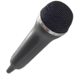
Since the sound has to travel out from speaker to object, then back to the microphone, the distance can be calculated as approximately $\frac{1}{2} \times \text{time taken} \times \text{speed of sound}$ (assuming speaker and microphone are relatively close together).

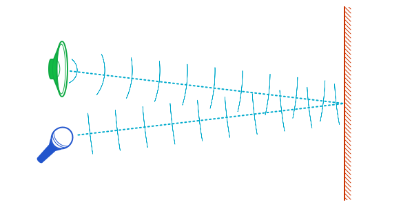
The speed of sound in air can be approximated as 343m/s ±5%^{(note 1)}, so if our microphone picks up the sound 5ms after the speaker made it, the soundwave must have travelled about 1.72 metres in total (round-trip), meaning the object is 86cm away (±4cm)^{(note 2)}.

This equation can also tell us how granular our answer will be: if we can determine the time to within a millisecond, then we can calculate the distance with ~17.2cm granularity (plus the overall 5% margin of error from variation in the speed of sound). Most computers use an audio sample rate of either 44.1kHz or 48kHz, so if we can get to-the-sample precision in our timings (~0.02 milliseconds), we can expect a distance granularity of 3.9 or 3.4mm, plus the overall 5% margin of error^{(note 3)}.

Dedicated hardware

Hardware which performs this exact operation is readily available, such as the HC-SR04, and typically advertises accuracy of “up to 3mm” (theoretically requiring a sample rate of at least 60kHz).

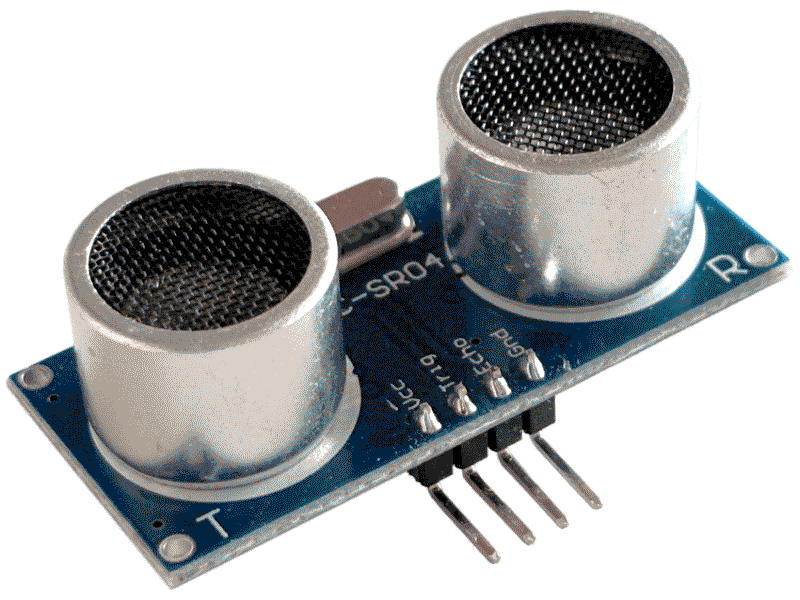
This specific example sends out a series of 8 very short 40kHz beeps (which requires a digital sample rate of at least 80kHz due to folding). The beeps are inaudible to humans, since the human ear is unable to detect sounds above ~20kHz, but is audible to (for example) dogs, cats, and mice. It then listens for the first echo which matches the same pattern of 8 pulses, and reports the time elapsed.

Can we do better?

Dedicated components have the advantage of directional speakers / microphones, and very high sample rates, but they have minuscule processing power and only report a single reading: the time to first echo. Echoes contain much more information: they can reflect back from different directions, and at each boundary some of the soundwave’s energy will continue into the object rather than reflecting back. Objects will also absorb and reflect different frequencies in different proportions due to resonance. These behaviours mean we should be able to see multiple reflected echoes, and can say something about each object’s properties based on how strong the echo is at different frequencies. Doppler shift means we can even identify the relative speed of the detected objects.

Signal

The first thing to notice is that if we wish to pick up more than one echo, we’ll need to use a more complicated signal than a fixed-tone beep. The sounds are likely to be so close together that they overlap, which will be impossible to distinguish if they are all the same frequency:

Here it is useful to look to nature. Bats use a sound known as a “chirp”. This is a sound which starts at one frequency, then sweeps to another frequency over time. As the echoes come back staggered over time, their frequency separation makes them much easier to distinguish:

Different species of bat have different sounds; the frequency range, duration, and harmonics all vary. Some species even include a fixed tone in the middle of their call (which they can use to detect relative velocity of the target object via Doppler shift). Hunter Scott’s The DSP Behind Bat Echolocation has spectrograms of a wide selection of real bat recordings, illustrating how much variety there is.

Many bat species’ calls contain a chirp which uses a hyperbolic curve in frequency space, rather than being linear:

The advantage of such a curve is that it is not distorted by Doppler shifting, which means the echo can be detected in the same way regardless of relative velocities (very useful for a creature in flight).

It also has the nice property that higher frequencies account for proportionally less of the signal. This means that if our signal is low-pass filtered at any point (either intentionally by the speaker or microphone, or as the result of hardware limitations), only a small part of it will be lost and we should still be able to detect it reliably (though at a cost to the temporal accuracy).

We don’t have to be constrained to nature, or even to lines:

So if we want to have some fun we could try locating things by bouncing smiley faces off them.

For our purposes, the properties of the hyperbolic chirp make it a good choice for getting started, even if we later revisit it to use something more fine-tuned to the situation. To avoid sharp “clicks” at the start and end of the chirp, we can use a simple linear “fade in” and “fade out”; this article uses a 1-millisecond fade in, and a 2-millisecond fade out.

Detection

Having an easily detected signal is all well and good, but how do we actually detect it?

One approach would be to calculate a spectrogram from the microphone (like the illustrations in the previous section) then use image analysis to locate the shape of our signal. There are well known and efficient ways to find a known shape in an image (e.g. Haar cascade classifiers), and once we find it we can easily analyse the image to see which frequencies have been absorbed (allowing us to do some rudamentary object classification). We can also subtract each signal after we find it and search again to find the next echo, even if they were overlapping. However, there is also a big disadvantage to this approach: performing frequency analysis involves a trade-off of frequency precision vs. time precision (due to the equivalent of Heisenberg’s uncertainty principle)^{(note 4)}. This significantly reduces our distance accuracy. Ideally, we would like to be able to identify echoes with sample-level precision.

The solution to this problem is simple and elegant, but needs some introduction.

Convolution

Suppose we wanted to go the other way: given a clean timeline showing the instants and intensities of the echoes, as well as our signal, we want to generate the audio which we would expect to hear. This process is called “convolution”, denoted $A * B$, where $A$ and $B$ are arrays of values.

To get a sense for the operation, a convolution can be implemented naïvely in Python as:

def convolve(A, B):
  result = [0 for i in range(len(A) + len(B) - 1)]
  for i in range(len(A))
    for j in range(len(B))
      result[i+j] += A[i] * B[j] # note: this * is regular multiplication!
  return result

If $A$ and $B$ have length $n$, this has a computational complexity of $\text{𝒪}(n^2)$, which means it can slow down significantly as the length of the inputs increases. It is much more computationally efficient to use the mathematical identity:

Where $ℱ$ is the fourier transform and $\otimes$ denotes element-wise multiplication^{(note 5)}. This identity lets us implement a convolution as:

def convolve(A, B):
  fA = fft(A)
  fB = fft(B)
  for i in range(len(fA))
    fAB[i] = fA[i] * fB[i]
  return ifft(fAB)

Where fft is some implementation of the “Fast Fourier Transform”, and ifft is the inverse; libraries with these functions exist for most programming languages.

Our $A$ and $B$ inputs must now have the same size, and depending on the Fast Fourier Transform implementation it may need to be a power-of-two, but there are techniques to avoid these limitations (discussed in part 3). For now we can pretend that it’s as flexible as the naïve approach.

The computational complexity of the Fast Fourier Transform is $\text{𝒪}(n \log(n))$, so this is more efficient, but the part which is interesting to us is is not the speed; it is that we have turned a summation over many elements into a simple element-wise multiplication, and element-wise multiplication is reversible.

Deconvolution

Rearranging the above equation, we can see that:

Where $\oslash$ denotes element-wise division. This lets us “undo” the convolution which has been applied! The operation is known as “deconvolution”.

If $B$ is our chirp, and $A * B$ is the audio received by the microphone, then we can use this to find the clean timeline of echoes which we are looking for ($A$).

Since we need to perform this operation a lot, and the chirp ($B$) does not change, we can also pre-compute $B_{\text{inv}} = 1 \oslash ℱ(B)}$ which lets us use multiplication rather than division in our loop for a small speed boost. The result of the fourier transform is actually an array of complex numbers, so calculating this inverse for each element is not quite as trivial as it could be, but it is still very easy:

Where:

• $b^{*}$ is the complex conjugate: $\text{Real}(b) - i \text{Imaginary}(b)$
• $\left|b\right|$ is the norm (i.e. length) of $b$: $\sqrt{\text{Real}(b)^2 + \text{Imaginary}(b)^2}$

Written as code:

def complex_reciprocal(z):
  m = 1 / (z.real ** 2 + z.imag ** 2)
  return complex(z.real * m, -z.imag * m)

(of course in real Python code you could simply write 1/z, but this is to illustrate the process using basic operations).

Dividing by 0

Division has a problem: If $b$ is 0, the division will explode. More generally: the accuracy will degrade as $b$ approaches 0. In practical terms, this means that noise at frequencies which are not used by our chirp will cause large errors in our output.

We can work around this by adjusting the equation so that it can never result in a division by zero:

This may look like a hack, but it actually has theoretical backing. In the optimal case, $c$ is a function of frequency: $c(f) = \frac{1}{\text{SNR}(f)}$, where $\text{SNR}(f)$ is the signal-to-noise ratio calculated for a given frequency. To calculate these values we can look at the audio received by the microphone when there is no echo expected (e.g. just before we send out our signal), fourier transform it, and compare each frequency bucket with the fourier transform of our signal (both squared because we want to know the ratio of energy rather than amplitude):

There’s still a free constant $v$ (related to volume, since we don’t know how loud our signal will be when it is emitted), but this no-longer depends on the frequency so we can tune it quite easily with trial-and-error.

Combining these equations, we can simplify some terms:

Or if we’re feeling lazy, we can skip the SNR calculation entirely and just approximate $c$ as a constant: values around 1000 work quite well (this corresponds to a SNR of -30Db, reflecting the fact that many frequencies do not occur at all in our signal).

Cross-correlation

Some sources use “cross-correlation” rather than deconvolution to detect echoes. The two approaches are very closely related: the process is the same, but cross-correlation replaces $\frac{1}{b}$ with $b^*$ in the inversion above; dropping the denominator $\left|b\right|^2 + c$ entirely. This means it can be turned into deconvolution by applying a collection of specifically-tuned band-passes to the input first.

In practice, using cross-correlation on its own (without these band-passes) is workable, but gives less focused results, making it more difficult to distinguish echoes from the noise and interference patterns. Deconvolution has the same performance (if we precompute $B_\text{inv}$ as noted earlier) and gives better results even when using approximated noise levels.

Simulating detection

If we can’t detect echoes in a perfect simulated environment, we don’t stand a chance in the real world, so let’s see how this deconvolution technique performs with our simulated environment from above:

It identifies the echoes with good precision. From this data we can find the echoes programmatically with a simple heuristic:

For each sample (ordered by time):
- If the sample is larger than any others within a 0.2ms window:
  - If we do not yet have a threshold:
    - we have found the immediate feedback peak;
    - set the threshold to the current sample value * 0.01;
    - continue to the next sample.
  - Otherwise, if the sample is greater than the threshold:
    - record an echo at time = current_sample_index / sample_rate.

This finds both echoes, and positions them at 2.333ms and 3.500ms^{(note 6)}. These are very close to the true values of 2.337ms and 3.502ms (within 0.2%).

As a comparison, let’s see what the same technique finds if we use a flat tone instead of a chirp:

The echoes are still there, but it is struggling to localise them. This represents a fairly extreme example: our signal is quite long and has not finished being sent by the time these echoes return (meaning we have a lot of interference), but it demonstrates how much our choice of signal impacts the system. Let’s stick with a hyperbolic chirp for now!

Sub-sample precision

We can get even more precise distance estimates by fitting a quadratic polynomial using the samples to the left and right of each peak (using Lagrange polynomials) and differentiating it to find the maximum point of the curve:

Starting with the Lagrange polynomial definition:

We can calculate the polynomials for a 3-point quadratic with points at $x$ = (-1, 0, 1):

Multiplying each of these by the value at that point ($v_{-1}$, $v_0$, and $v_1$), and collecting terms:

Differentiating with respect to $x$:

Equating this to 0 to find the turning point (maximum):

Plugging in our measured values for $v$ tells us the amount we need to shift the sample by for sub-sample precision (the resulting $x$ will be between -0.5 and +0.5).

For this experiment, the sub-sample adjustment moves our echo readings to 2.336ms and 3.501ms^{(note 7)}; both correct to within 0.05%. In the real world we expect noise to make our accuracy much worse, but achieving this high level of accuracy in an ideal simulated environment indicates that the approach is viable.

Inferring reflection intensity

You may have noticed in the previous section that the second echo has a lower amplitude than the first, even though both represent 100% of the signal being reflected. Specifically the detected intensities are 0.028 and 0.021^{(note 8)}. This presents a problem if we want to know how much sound an object actually reflected (e.g. to check if its surface is rough or smooth), so we need to model the phenomenon and adjust for it.

As a sound wave expands, the total energy of the wave stays the same^{(note 9)}, which means the energy of the wave in any given direction decreases in proportion to the total area covered by the wavefront. For a simple scenario where the sound wave is unconstrained and can travel in all directions, this tells us that $E \propto d^{-2}$, where $E$ = energy in a given direction, and $d$ = distance travelled^{(note 10)}.

We don’t directly have the energy ($E$) or the distance ($d$), but for sound waves $E \propto A^2$ (where $A$ = amplitude); and in any given environment the speed of sound in air stays relatively constant: $d \approx v t$, where $t$ is the elapsed time, and $v$ is some unknown but constant velocity^{(note 11)}. Put another way: $d \propto t$.

Combining all of these relations, we can say:

The constant of proportionality does not matter to us, since the user may have an unknown gain level (volume) on their speakers and microphone anyway, so for our purposes we’ll just say the constant is 1^{(note 12)}.

Applying this per-sample scaling to our simulation (after performing the deconvolution), we get spikes which are of a consistent size:

The detected intensities are now 0.227 and 0.246; within 10% of each other (this remaining difference is probably due to inaccuracies in the deconvolution, and the fact that a quadratic curve is not a perfect fit for the data).

Note that for this to give accurate results, we must ensure that the measured time is “like for like”: if our deconvolution is giving us the midpoint of detected samples, then we must measure time from the midpoint of the emitted sample, not the moment we started playing it.

Latency

Outside our simulation, we have a problem: we do not know exactly when the chirp was emitted from the speakers, nor do we know exactly when the microphone picked up its echo. All we know is when we told the speakers to produce a sound, and when the microphone reported the sound to us. There is an unknown amount of latency on both sides.

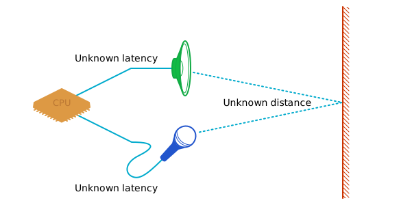
For fixed hardware, this is not a concern. We can simply measure the latencies in a known environment and hard-code them into our software. But if we want our program to work with arbitrary hardware and software stacks, then we cannot rely on knowing these latencies in advance.

The WebAudio API does include some latency reporting: if the browser supports the feature, it can tell us the predicted output and input latencies of a device. This may include software latencies (due to signal processing and queues) as well as hardware / firmware latencies (such as the time taken to send a signal to a bluetooth speaker). But these values are not guaranteed to account for everything, and they may not be available at all (especially if the user has external speakers with unknown characteristics). These are a good starting point when they are available, but they are not enough to solve the problem.

Error tolerance

So amidst all this uncertainty, how certain do we need to be?

Earlier in this article, we established that there is a fundamental error in echolocation distances of ±5% due to variations in the speed of sound. If we can’t measure the air temperature, pressure, or humidity, and we don’t have any points of comparison to calibrate against, then it doesn’t matter how good our processing is: we cannot reduce this error. This gives us something to compare our latency-induced errors with.

Also, for our purposes, we don’t actually care what the speaker or microphone latencies are individually; we only care about the sum of these latencies. This reduces our problem to 2 unknowns (total latency, and distance to object).

If our latency estimate is out by 0.6ms, then we will have doubled the overall systemic error at 2 metres. At 1 metre, the threshold for doubling the error is just 0.3ms (equivalent to 14 samples at 48kHz).

We may also want to consider the impact on our reflection intensity normalisation. We can compare our example echoes at 40 and 60cm:

In this case, underestimating the latency is significantly better than overestimating it; an underestimation of 2ms results in an 18% error in the relative intensities, but an overestimate of 2ms introduces a 65% error.

The next article will discuss how we can use measurements from multiple components to infer latencies automatically (if we have enough components available).

Free parameters

We’re left with a few free parameters which we can experiment with:

• The latency estimate controls distance calculations and relative intensities of the detected echoes;
• The signal-to-noise ratio of our emitted chirp is used in the deconvolution, and controls the sharpness and noisiness of the resulting detections;
• The frequency range of our chirp can be tuned to the maximum within the abilities of the hardware (e.g. based on the available sample rate, and whether it applies band-passes to the speaker and/or microphone);
• The direction of the chirp (increasing or decreasing pitch) makes no difference to the mathematics, so can be set to whichever sounds least irritating;
• The duration of the chirp controls how far we wish to look: longer chirps make it easier to detect faint echoes from long distances, whereas short chirps interfere less with echoes which come back quickly from short distances (as a point of reference: many bats use chirps around 4ms in duration).

Next steps

We have a way to get 1-dimensional data about multiple object positions by using echolocation, and we can classify these objects somewhat based on their reflectivity. Part 2 (not yet posted) takes these results a step further: inferring 2-dimensional positions of objects when multiple speakers and/or microphones are available. Part 3 (not yet posted) shows how to build these techniques into a browser-based application.

Further reading

• The DSP Behind Bat Echolocation
• Animal echolocation on Wikipedia
• Fourier transform on Wikipedia